Project Results

This video is a quick review of interpreting your reports in the packet.

Presentation 

The following presentation is provided in both video and in text.

This presentation provides group findings in addition to those found in your individual packet of information. This information is supplementary to the packet you received, so please do not rely entirely on this presentation as the complete summary to your department's results.

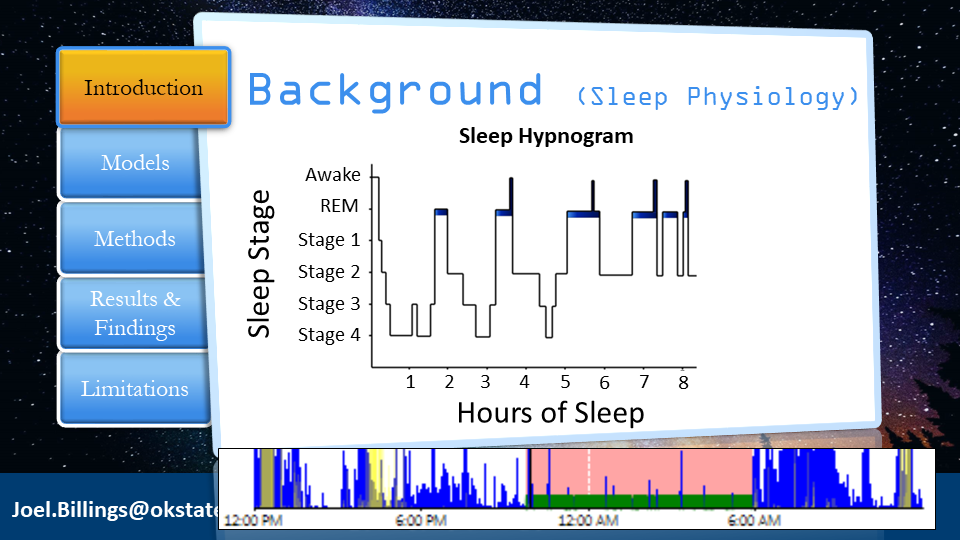
This figure illustrates a typical sleep pattern (called a sleep hypnogram) for an average individual that experiences one sleep bout. Notice that the y-axis represents the different stages of sleep with deep sleep being in stages 3 and 4. The x-axis represents the number of hours of sleep. The idea here is to see that this pattern changes throughout the progression of sleep. So, essentially, we are studying what happens when this patter becomes fragmented by responding to calls and sleeping at the station.

These are samples of sleep actigraphy taken from a few participants. In the top sample, the participant went to bed around 12:00am (indicated by the pink and green). He experienced a call, came back and fell asleep, experienced another call, and then came back to the station and fell asleep again. The second illustrates one falling asleep just before midnight. He received a call and after returning back to the stations, he could not return to sleep. The third sample is a mix. This individual attempted to sleep early, but was awoken and went on a call. He came back to the station and tried to sleep, but experienced a lot of activity (e.g., tossing and turning) before ending sleep at 6am. As a result of fragmented sleep, many participants experienced sleep as illustrated in the last sample. Here, this individual slept for a significant duration on the first night following the end of a shift.

The results of my previous study (2014) found no statistically significant difference of sleep quality scores between the 24/48 and 48/96 shift schedule. However, the study had a few limitations, residing mainly with control variables. Therefore, this dissertation research reexamines these two schedules using a better method (i.e. experimental design).

Two approaches were adopted to examine sleep quality. The first approach was subjective (i.e., the Pittsburgh Sleep Quality Index), which is a quick survey that, in general, provides a rough insight on one's sleep quality. The second approach was objective, which captured the data automatically via the activity watch you wore throughout the study periods. This objective approach reduces data error by nearly eliminating any guessing work in your sleep times.

This image illustrates a flow of participation throughout the study (note: you might have to click on the picture to see the details). The study ended with a total of 24 participants with eligible data to analyze.

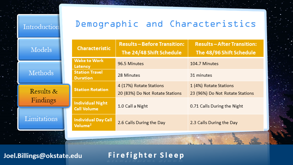
These three slides provide demographic and characteristic information. Note that individual call volume during the night decreased after the transition. This will help explain some of the sleep results in the later slides.

The first approach used the PSQI. The raw PSQI results indicate that 9 out of 24 participants had poor sleep quality during the 24/48 and increased to 11 out of 24 participants during the 48/96 schedule.

This is a regression model where the control variables come into the equation. These variables are important because they help eliminate their influence on sleep so that the results reflect the main independent and dependent variable. For example, we want to control "station number" (and more specifically number of calls) because if one person moved from a non-busy station to a busy station, we would expect their average sleep duration to decrease. Without including this control variable, the results would suggest that sleep quality decreased as a result of the schedule change. This, of course, is not necessary the result of the schedule, but likely due to the increased call volume after transitioning from a non-busy station to a busy station. This is why each participate completed the lengthy survey at the beginning of each round!

Now that all variables are controlled, the results of the regression model show that the sleep quality scores worsened at a statistically significant level after the shift schedule transition. In other words, this subjective approach found the 48/96 worse than the 24/48 shift schedule regarding sleep quality.

 

The second approach uses objective data recorded from the activity watch. This includes total time in bed, total sleeping time, sleep efficiency, sleep latency, number of awakenings, minutes awake after sleep onset, steps, and activity level.

This table details each raw sleep parameter in different categories (home, work, and overall tour) for each round (note: you may have to click the image to view detail). Most of the parameters improved slightly. However, most increases were not statistically significant, meaning essentially no difference.

This is the regression model for the second, objective approach where control variables are included. The results suggest no statistically significant difference exists between sleep quality and shift schedule. In other words, we found no differences in sleep between the schedules.

To recap, the first approach found a difference in scores. However, several limitations in the instrument are noted and therefore, find the applicability of the PSQI not best suited for the fire and emergency services. The second approach did not find statistically significant differences in the sleep quality scores between the schedules. This discovery warrants explanation.

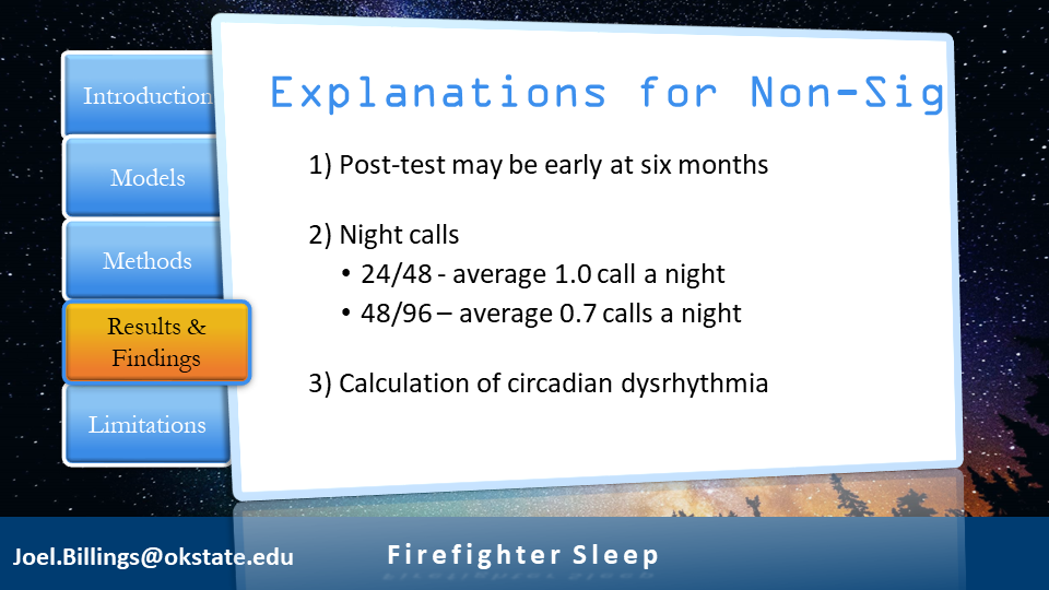
A few explanations exist for the absence of a statistically significant relationship. 1) Six months may be too short of a study duration. This is especially important when thinking about long-term health effects that take longer than six month to display any notable differences. 2) Individual night call volume decreased on the 48/96 shift schedule. A decrease in interruption (e.g., responses) provides greater opportunity to sleep.

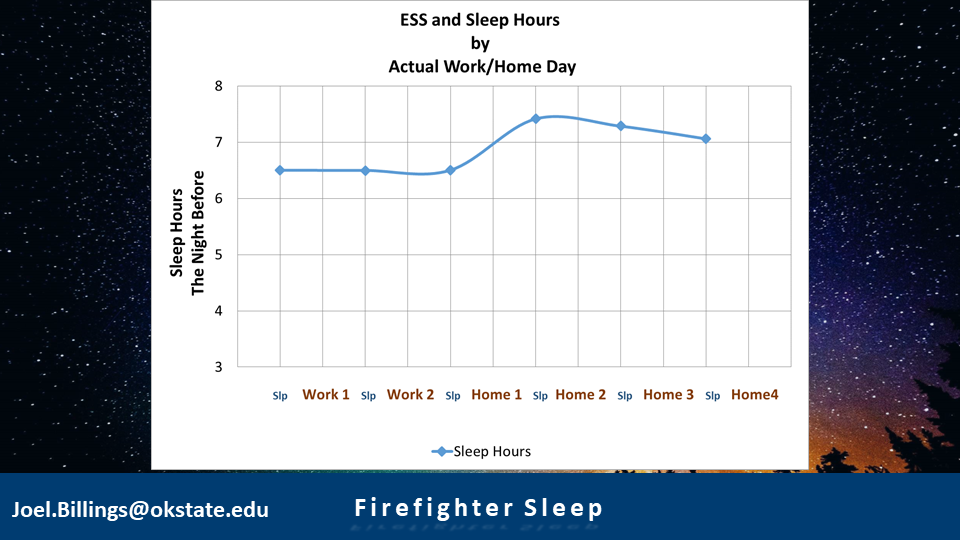
3) Perhaps the calculation of circadian disruptions associated with each schedule needs adjustment. These two charts show the actual sleep hours for each day in a tour between the 24/48 (top) and 48/96 (bottom). The least amount of sleep in both schedules was recorded the night prior to going to work. Previously, this was believed to equate to a 'good night of sleep' whereas now, these results would suggest the night prior to work equates to a 'poor night of sleep'. Therefore, assuming all work nights are still considered poor, the calculation becomes slight different. For the 24/48, 2 out of 3 (66 percent) nights are considered poor. For the 48/96, 3 out of 6 (50 percent) nights are considered poor. This, of course, need more research.

4) Responsibility can be modified to allow rest and sleep. While not necessary specific to the department under review, most department that elect the 48/96 develop a contingency policy to allow rest and sleep. For example, members can sleep-in during the second workday, members can rotate to less busier stations, and different stations can be toned-out should a particular busy station become fatigued with night calls. 5) Sleep duration can likely increase due to the reallocation of the previous wake-to-work latency. Members typically woke 100 minutes before shift start time during their first shift. Considering no travel on the second 24 of the 48/96, members typically extended their sleep. This, of course, provided more sleep opportunity and reflects in the data results. If the 48/96 was comprises of two exact 24/48 shifts, meaning wake up early when commuting to and from work, we would expect sleep to decrease. However, since commute (and likely prepping for work) is halved, sleep opportunity increases.

Two main implication resulted from this study. Regardless of shift schedule, firefighters in the study averaged an inadequate sleep duration. One intervention is to nap (or allow naps) when appropriate. [ Visit the research section of FDSleep.com to read research on napping - and of course, napping is not a substitute for sleeping]. The second intervention is shift start time. In the chart above, the least amount of sleep occurred during the night prior to first workday. The second least amount of sleep occurred during the second work night. It is believed that this is due to waking up early to prepare and commute to work and then waking early to prepare to go home. This relationship occurred during both schedules.

Waking up early reduces sleep opportunity. If shift start time was adjusted back, personnel would have an greater opportunity to increase sleep before going to work and returning home. Further, depending on the start time, benefits would extend to avoid rush hour commutes and allow those with children to drop them off at school. [Visit the Research section of FDSleep.com to view information on Shift Start Time] It is believed that adjusting shift start time to later in the morning may reflect actual sleep hours shown in the graph below. This would be one, critical step forward helping to increase sleep duration.

As with most studies, limitations exist that impact the results (and interpretation therein). The results of this study cannot be generalized (transferred) to any other department. The study concluded with 24 participants having eligible data. A greater sample size is needed to have generalizable results. Furthermore, it is unknown how those who did not participate would influence the results. Another limitation is study duration. Six months is probably not sufficient to allow chronic effects to register any significance. Future studies should examine departments with different number of personnel, individual call volume, and shift schedules.

Another limitation exists in the Sleep Quality Model (SQM), where it was not previously validated. In addition, other instruments used to measure control variable may also have limitations affecting the generalizability of the results.